DM(X)

Today I discovered a very nice Analysis Services client tool. Produced by SQLMinds, the tool seems a great addition to Analysis Services. It provides many components, among them a performance tuning service, an OLAP cube browser for the web and a very nice web front end for data mining, the DM Companion tool which can be launched at http://x32.sqlminds.com/dmcompanion.

So, here are a few really nice things about the DM Companion tool (BTW, a fully working demo is running at the aforementioned URL).

The tool works to some extent like a Data Mining -specific SQL Server Management Studio for the web. Therefore, it allows you connect to the server of your choice (through the Analysis Services HTTP pump). The demo seems to allow anonymous connections (pretty safe  as all the interactions offered by the tool are read-only).  Next you get to chose your AS catalog and the mining model you want to use.

For each model you have the option to browse the content or execute predictions.

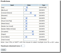
The prediction feature provides a nice interface for defining singleton predictions, as you can see below:

The interface supports specifying multiple nested table keys as input, so the tool can perform associative predictions as well. It reminds me of the XMLA Thin Miner sample running on SQLServerDatamining,com, however, it looks much better and is nicely integrated with the rest of the application. While prediction functions do not seem to be directly supported, the application is able to predict a cluster for clustering models.

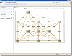
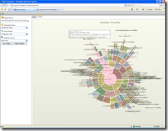
The model browsing features are really nice. Analysis Services includes a set of sample web viewers for Naive Bayes, Trees and Clustering. This application provides some seriously better looking viewers for these algorithms, and extends the suite at least for Neural Networks (a really nice viewer), Sequence Clustering and Association Rules.  The DM Companion viewers offer all the features in the sample viewers, with a nicer implementation which uses AJAX and has better graphics, plus a solid set of new features, the most spectacular being the interactive dependency net browser and the pie chart visualization for decision trees, which you can see below.

Overall, DM Companion looks like a really nice tool for sharing your data mining implementation on the web

Tags: DMX by bogdan
4 Comments »

Some very interesting, although time-consuming project kept me away from posting in the last month. Mea maxima culpa, I will try to catch up and put some new and interesting content here more often.

Recently, trying to make sense of some prediction results, I realized that the DMX NATURAL PREDICTION JOIN statement has some obvious and some not so obvious dangers, which deserve some clarification.

To summarize, the PREDICTION JOIN operator is used to apply patterns from a trained mining model against new data. The general syntax is

SELECT EducationLevel

FROM MyModel

PREDICTION JOIN

OPENQUERY(MyDataSource, ”SELECT Height, , HairColor, ShoeSize FROM CustomerInfo’) AS T

ON

T.Height = MyModel.Height AND

T.HairColor = MyModel.HairColor AND

T.ShoeSize= MyModel.ShoeSize

In the standard PREDICTION JOIN statement, the ON clauses specify how columns from the new data are to mapped to the input columns of the mining model.

The statement supports a simplified format:

SELECT EducationLevel

FROM MyModel

NATURAL PREDICTION JOIN

OPENQUERY(MyDataSource, ”SELECT Height, HairColor, ShoeSize FROM CustomerInfo’) AS T

In the simplified format, the columns from the new data are mapped to the input columns of the mining model by name. Much easier to type, resulting in a more readable statement!

Now, the natural mapping may end up in three different scenarios. In the first scenario, all the model’s input columns find a corresponding data column in the input. The mapping is performed correctly and everything works as expected. Nothing to blog about in this case!

The second case: some of the inputs are mapped correctly to model columns, some are not, although you would expect them to be mapped correctly. More than a simple user error, this situation is actually “facilitated” by the way the BI Dev Studio works. Assume you start with a table containing 4 columns: Height, HairColor, ShoeSize, EducationLevel and use BI Dev Studio to create a mining structure and a model. BI Dev Studio will generate more friendly names for the columns and your mining model ends up with the structure below:

MyModel

(

Height

[Hair Color],

[Shoe Size],

[Education Level]

)

[Read more →]

Tags: DMX by bogdan
1 Comment »

This an actual question I had to answer in one of the previous Tech Ready conferences: when does one know that feeding more data to the mining model will stop improving accuracy? Or: how much training data is enough? With the new accuracy procedures in SQL Server 2008, I think I have now a better answer.

Algorithms learn from data and, generally, feeding them with more data will improve the accuracy. This improvement, however, is asymptotical. If the training data is statistically representative for the problem space, then a classifier will stop learning after a certain limit: new data points will support existing patterns and will help reducing the risk of over-training,  but will not add more information to the model. The solution I suggest for SQL Server 2008 allows you to figure out if your mining model is likely too gain from adding new data or is likely to maintain the same accuracy.

The solution is based on the cross validation mechanism, so I’ll start with a small presentation of this mechanism. The cross-validation takes a data set, splits it into a number of (roughly equal size) partitions, called folds, then builds a set of mining models (as many as there are folds). Each mining model is built on top of the whole data set minus one of the folds and then the accuracy of the model is measured on the fold that was left out. Effectively, all data is used in training and all data is left out (by at least one mining model). Also, each model is validated against data that was not seen during training. The accuracy measures for each model are then evaluated across all the folds. A good mining solution would provide compact accuracy measurements (i.e. no big differences between the measurements on different folds). Spikes in the measurements may indicate problems with the data. Note that cross validation does not improve the accuracy of the model, it just provides an “honest” estimation of that, reducing the risk of over-training.

In SQL Server 2008, cross validation allows the user to specify how many cases should be used for the procedure. This is mainly for performance purposes — it allows a quick comparison between different mining models/algorithms on the same data set.

Now back to the original problem: would adding new data benefit the accuracy?

[Read more →]

Tags: 2008, DMX, SQL Server by bogdan
No Comments »

This second post on model filtering deals with nested table filters. The most common use of nested tables in SQL Server Data Mining is to model transaction tables. That is, model Customer entities together with the “bag” of products they purchased.

Nested table filters primarily serve two purposes:

• - Use (in the model) only those nested table rows with a certain property (e.g. consider only products that are not “Coca Cola”, because most people do buy “Coca Cola”, so it is not that interesting)
• - Use (in the model) only those cases where the associated nested tables have certain properties (e.g. - build a prediction model on customers that have purchased Coca Cola)

Notice the difference between the filters: while the first filter removes products from shopping baskets before modeling, the second removes customers from the model (those that have not purchased Coca Cola).

[Read more →]

Tags: 2008, DMX, Modeling, SQL Server by bogdan
1 Comment »

This is the first post in a small series describing my favorite data mining feature in SQL Server 2008, model filtering. Filtering allows you to take full advantage of the mining structure / mining model dichotomy, separating the data staging (in the structure) from the modeling (in the mining model).

SQL Server 2008 allows specifying, for each mining model, a filter to be applied on the training data. The filter acts as a partitioning mechanism inside the mining structure and it is applied on top of any training/testing partitioning already existing at the structure level.  Furthermore, filters can be applied to data in nested tables, but more about this in the next post. Filters allow you to build different models for various partitions of the data with minimal effort, either to obtain better overall accuracy (think of it as manually specifying the first split in a decision tree), or to compare the patterns between different partitions.

So, let’s start with a simple scenario, using the same old Adventure Works data - building a mining model that predicts how likely a customer is to purchase a bike based on various demographic information. Let’s also assume that you know, based on your experience with the data that the Geography factor has in important role and you don’t want your North American patterns to hide (because of volume) the peculiarities of the Pacific market.

Suppose you start with a mining structure defined like below:

[Read more →]

Tags: 2008, DMX, SQL Server by bogdan
No Comments »

In a previous post I presented some of the new DMX features in the November CTP of SQL Server 2008. So, here are some new cool DMX tricks.

Assume you want to use Microsoft Association Rules and Microsoft Decision Trees on the same data. Also, assume that the data contains one numeric column (say, Age). You may have noticed that Decision Trees supports continuous columns, while Association Rules does not. Not a big deal, we have discretization, and Age can be added twice to the same mining structure as, say Age (Continuous) and Age Disc (Discretized). However, the two different names raise a problem in the case of NATURAL PREDICTION JOIN (where input columns are bound by name to the model columns).

In SQL Server 2005, the mining model columns typically had the same name as the mining structure’s ones. There was no way in DMX to change the model column names (well, there is a way in BI DevStudio).

Another problem: one would not include the email, name or phone number of a customer in a mining model, because, at best, this would increase training time and, in the worst case, would unnecessarily complicate the model with fake patterns. But this makes it hard to link the training cases leading to one pattern (available with the drillthrough feature) to information that would perhaps make that pattern actionable (like contact information, if the pattern suggest strong probability to buy a product).

In 2008, these problems are much easier to solve, with mode column aliasing and structure columns drillthrough, and here is how these work.

[Read more →]

Tags: 2008, DMX, SQL Server by bogdan
1 Comment »

As Raman mentioned in the Data Miner newsletter, the November CTP of SQL Server 2008 is now available.

It includes many really cool new features in Analysis Services. Among them: Holdout support, Model filtering, DMX Column aliasing, Drillthrough enhancements, Cross validation and practically two new forecasting algorithms under the Microsoft_Time_Series umbrella.
I intend to present all of them briefly, and I start today with the Holdout support.

Most of the data mining tasks require a validation step, performed right after modeling. This validation step
consist (typically) in evaluating model’s performance against data that was not seen during training (test data). 

The test data ideally has the same statistical properties as the training data (data seen by the mining model during training). An easy way to achieve statistical similarity between the training and test set is to use random sampling. This method is not guaranteed to give correct results (statistical similar populations) but, assuming that the random sampling mechanism is independent of the data, it will work in most common scenarios.

SQL Server Integration Services has a Random Sample transform, which extracts a random sample (with a certain percentage) using a mechanism independent of the actual data being samples. This is why we strongly recommended using Integration Services to generate test/training partitions for SQL Server Data Mining.

However, there are a few problems:
- Integration Services will have to save at least one of the sample sets in a relational table (or some form of output destination)
- This sampling method can only be applied to data coming from a relational source (or, in general, a source that can be used with IS). That means it is difficult to use IS sampling with application that do data mining on in-memory data
- Integration Services is rather hard to use to sample data for models with nested tables. It can be done, but it takes around 11 simple steps and 14 transforms to do this for a single nested table (an example is available here: Sampling Nested Tables )

Now, there is a simpler way to do this. You may remember that, in the SQL Server Data mining architecture, a Mining Structure object acts as a data space while a mining model is a problem to be addressed in that data space. As the mining structure describes the data space, it is  natural for the structure to partition the data into training and testing sets.

In SQL Server 2008, the new wizard for creating a model (or structure — yes, there is a wizard now for creating a structure with no models!) allows specifying the desired size of the “Holdout” dataset — that is, data to be stored in the mining structure for testing purposes, without being available for models training. By default, the holdout size is 30% (leaving 70% for training). You may choose to specify a fixed number of rows instead of a percentage, or both (in this case the semantic is “use 30%, but no more than 10000 rows for test data”).

The rest of this post shows how to express the holdout wizardry in DMX.

[Read more →]

Tags: 2008, DMX, SQL Server by bogdan
1 Comment »

A recent post on the MSDN Forums raised an interesting issue: Excel Data Analysis’s Linear Regression and SSDM were returning different results. Specifically, the SSDM results were much worse.

The issue turned out to be a data modeling issue (columns were not mapped properly).  However, during the investigation I had to compare Excel’s linear regression with the SSDM regression algorithm(s). Thought this might be interesting, so here is one way to compare the results from the two implementations.

I started with some simple (X,Y) data (available for download as a CSV file). First step - run Excel’s Data Analysis regression tool. The results are displayed typically in a separate spreadsheet, and the interesting part  is the Coefficients sections:

Therefore, the Excel regression formula is
Y = 2.37486095661847*X -0.310344827586214

Next thing — apply Excel’s regression coefficients to the existing data. I did this by adding a column in my data spreadsheet and populating it with a formula:

Next thing, I created a Microsoft Linear Regression mining model on the same data. There is a variety of ways to do this, such as exporting data to a table, connecting directly to the Excel spreadsheet or, the simplest way, by using the Excel add-ins.

To get the model’s predictions in Excel, I used one of the functions exposed by the Excel add-ins, DMPREDICT. If you do not have the add-ins you can always execute a prediction query in SQL Server Management Studio or BI Dev Studio.
However, with the add-ins’s function, getting the prediction results is really easy:

[Read more →]

Tags: DMX, Excel Add-ins by bogdan
2 Comments »